Fabric RTI 101: Trend Analysis in KQL

Trend analysis is one of the most powerful applications of KQL — it lets you move beyond simple metrics and start understanding how your data evolves over time.

Most trend analysis begins with the make-series operator. This operator constructs a time-series dataset by grouping values into evenly spaced time intervals. You might, for instance, calculate the average response time or error count every minute, hour, or day.

Here’s a simple example:

Requests
| make-series AvgResponseTime = avg(DurationMs) on Timestamp in range(ago(1d), now(), 1h)

This creates a new series showing average response times over the past day, in hourly intervals. The result is a dataset structured for time-based analysis — ideal for spotting peaks, dips, and patterns.

Once you’ve built that time series, you can use the render operator to visualize trends directly in your query results — for example, as a line chart:

| render timechart

Visualization helps make anomalies and seasonal trends immediately clear.

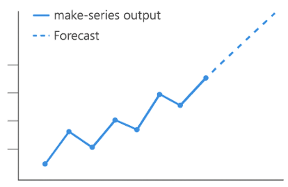
KQL also supports decomposition and forecasting functions, which let you break down a time series into its trend, seasonal, and residual components. That enables you to forecast future values based on past behavior — a capability that’s especially useful in proactive monitoring and capacity planning.

KQL isn’t just for reacting to what’s already happened — it’s for predicting what’s coming next. Trend analysis turns telemetry data into proactive insights, helping teams anticipate issues and optimize performance before problems occur.

Learn more about Fabric RTI

If you really want to learn about RTI right now, we have an online on-demand course that you can enrol in, right now. You’ll find it at Mastering Microsoft Fabric Real-Time Intelligence

2026-06-26